
MNIST handwritten number identification
The task is to build a model to predict handwritten numbers as accurately as possible.
Performance measures
Training a multiclass classifier
EDA and visualisation
from sklearn.datasets import fetch_mldata
mnist = fetch_mldata('MNIST original')
mnist
{'COL_NAMES': ['label', 'data'],
 'DESCR': 'mldata.org dataset: mnist-original',
 'data': array([[0, 0, 0, ..., 0, 0, 0],
        [0, 0, 0, ..., 0, 0, 0],
        [0, 0, 0, ..., 0, 0, 0],
        ...,
        [0, 0, 0, ..., 0, 0, 0],
        [0, 0, 0, ..., 0, 0, 0],
        [0, 0, 0, ..., 0, 0, 0]], dtype=uint8),
 'target': array([0., 0., 0., ..., 9., 9., 9.])}
X,y = mnist['data'], mnist['target']
print(X.shape)
print(y.shape)
(70000, 784)
(70000,)
There are 70000 numbers, each stored as an array of 784 numbers depicting the opacity of each pixel, it can be displayed by reshaping the data into a 28x28 array and plotting using matplotlib.
%matplotlib inline
import matplotlib
import matplotlib.pyplot as plt

some_digit = X[36000]
some_digit_image = some_digit.reshape(28,28)

plt.imshow(some_digit_image, cmap = matplotlib.cm.binary,interpolation='nearest')
plt.axis=('off')
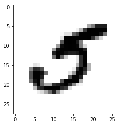
y[36000]
5.0
Section off a train and test set and shuffle them
X_train, X_test, y_train, y_test = X[:60000], X[60000:], y[:60000], y[60000:]

import numpy as np

shuffle_index = np.random.permutation(60000)
X_train, y_train = X_train[shuffle_index], y_train[shuffle_index]
Training a Binary Classifier
Identify a single digit, looking at 5s.
y_train_5 = (y_train == 5)
y_test_5 = (y_test == 5)
from sklearn.linear_model import SGDClassifier

sgd_clf =SGDClassifier(max_iter=1000,tol=1e-3,random_state=42)
sgd_clf.fit(X_train,y_train_5)

sgd_clf.predict([some_digit])
array([ True])
y[36000]
5.0
Simple to implement example in this case correctly predicting that the digit is a 5.
Performance Measures
Measuring accuracy using cross validation
Self implemented cross validation, allowing more control than sklearns readymade version.
from sklearn.model_selection import StratifiedKFold
from sklearn.base import clone

skfolds = StratifiedKFold(n_splits=3, random_state=42)

for train_index,test_index in skfolds.split(X_train, y_train_5):
    clone_clf = clone(sgd_clf)
    X_train_folds = X_train[train_index]
    y_train_folds = y_train_5[train_index]
    X_test_fold = X_train[test_index]
    y_test_fold = y_train_5[test_index]

    clone_clf.fit(X_train_folds, y_train_folds)
    y_pred = clone_clf.predict(X_test_fold)
    n_correct = sum(y_pred == y_test_fold)
    print(n_correct/len(y_pred))
0.95315
0.9674
0.9576
The stratifiedKfold class performs stratified sampling to produce folds that contain a representative ratio of each class. At each iteration the code creates a clone of the classifier, trains that clone on the training fold and then makes predictions on the test fold. It then counts the number of correct predictions and outputs the ratio of correct predictions.
from sklearn.model_selection import cross_val_score

cross_val_score(sgd_clf, X_train, y_train_5, cv=3, scoring='accuracy')
array([0.95315, 0.9674 , 0.9576 ])
The sklearn cross_val_score in action returning the same result.
print('95-96% accuracy is not as impressive as it sounds where there are {:.2f} percent 5s in the dataset'.format(sum(y==5)/len(y)*100))
95-96% accuracy is not as impressive as it sounds where there are 9.02 percent 5s in the dataset
Confusion matrix
The confusion matrix is a much better way to evaluate the performance of a classifier, especially when there is a skewed dataset as we have here with only 9% of the dataset being the target.
We first need a set of predictions to compare to the actual targets
from sklearn.model_selection import cross_val_predict

y_train_pred = cross_val_predict(sgd_clf, X_train, y_train_5, cv=3)
from sklearn.metrics import confusion_matrix

confusion_matrix(y_train_5, y_train_pred)
array([[53062,  1517],
       [  920,  4501]])
Each row represents a class, each column a prediction, the first row is negative cases (non-5s) with the top left containing all the correctly classified non-5s (True Negatives), the top right the 5s incorrectly classified as non-5s (False-Positves).
The second row represents the positive class, 5s in this case, bottom left contains the 5s incorrectly classified as non-5s (False Negatives), the bottom right containing the correctly classified 5s (True Positives)
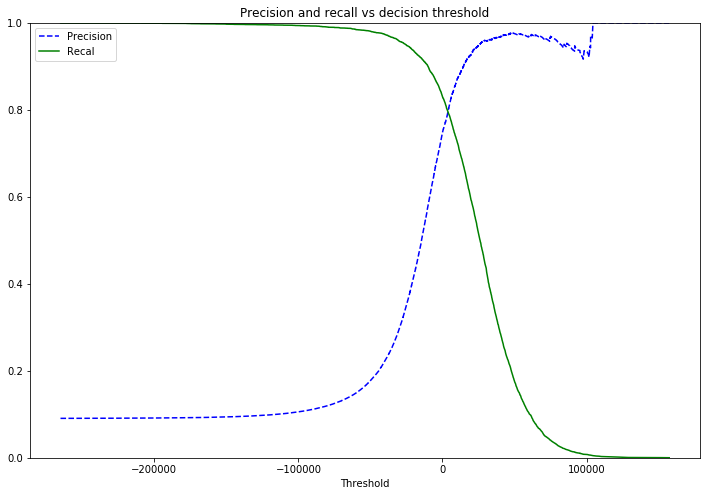
Precision/Recall
Precision measures the number of true positives (correctly classified 5s) as a ratio of the total samples classified as a 5. TP/ (TP + FP)
Recall measueres the number of true positives as a ratio of the total number of positives. TP / TP + FN
Depending on the scenario the model may be modified to try and maximise one or the other, catching all positive instances at the expense of catching some false positives. Or making sure a positive instance is never falsely identified as a negative at the expense of missing some of the positive instances.
y_scores = cross_val_predict(sgd_clf, X_train, y_train_5, cv=3,method='decision_function')
from sklearn.metrics import precision_recall_curve

precisions,recalls,thresholds = precision_recall_curve(y_train_5, y_scores)

def plot_precision_recall_vs_threshold(precisions,recalls,thresholds):
    plt.figure(figsize=(12,8))
    plt.title('Precision and recall vs decision threshold')
    plt.plot(thresholds, precisions[:-1], "b--", label="Precision")
    plt.plot(thresholds, recalls[:-1], "g-", label="Recal")
    plt.xlabel("Threshold")
    plt.legend(loc="upper left")
    plt.ylim([0,1])

plot_precision_recall_vs_threshold(precisions,recalls,thresholds)
plt.show()
The ROC Curve
The receiver operating characteristic (ROC) curve plots the true positive rate (recall) againt the false positive rate (negative instances that are incorrecly classed as positive). The FPR is equal to one minus the true negative rate, which is the ratio of negative instances that are correctly classified as negative. The TNR is also called specificity. Hence the ROC curve plots sensitvity (recall) versus 1-specificity.
To plot we need the TPR and FPR for various threshold values, using the roc_curve() function, we can then plot the FPR aginst the TPR.
from sklearn.metrics import roc_curve

fpr, tpr, thresholds = roc_curve(y_train_5,y_scores)

def plot_roc_curve(fpr, tpr, label=None):
    plt.figure(figsize=(12,8))
    plt.title('ROC curve')
    plt.plot(fpr, tpr, linewidth=2, label=label)
    plt.plot([0,1],[0,1],"k--")
    plt.xlim([0,1])
    plt.ylim([0,1])
    plt.xlabel('False positive rate')
    plt.ylabel('True positive rate')

plot_roc_curve(fpr,tpr)
plt.show()
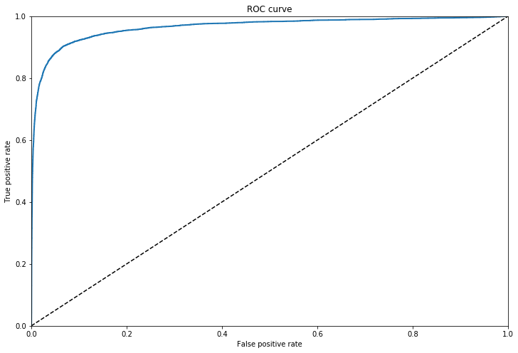
ROC AUC
Another way to compare classifiers is to measure the Area Under the Curve (AUC), a purely random classifier would have an AUC score of 0.5
from sklearn.metrics import roc_auc_score

roc_auc_score(y_train_5, y_scores)
0.9653891218826266
This score of 96% is misleading for problems in which the target class makes up a small percentage of the dataset. Looking at the precision recall curve makes it clearer that there is room for improvement, the curve could be much closer to the top right hand corner.
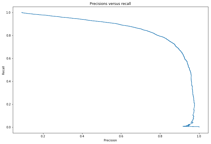
Precision recall curve
def plot_p_r(precisions,recalls):
    plt.figure(figsize=(12,8))
    plt.title('Precisions versus recall')
    plt.plot(precisions[:-1],recalls[:-1])
    plt.xlabel('Precision')
    plt.ylabel('Recall')

plot_p_r(precisions,recalls)
plt.show()
Comparison of models using ROC curves
from sklearn.ensemble import RandomForestClassifier

forest = RandomForestClassifier(random_state=42)

y_prob_forest = cross_val_predict(forest,X_train,y_train_5,cv=3,method='predict_proba')
y_scores_forest = y_prob_forest[:,1]

fpr_forest,tpr_forest,thresholds_forest = roc_curve(y_train_5,y_scores_forest)


plot_roc_curve(fpr_forest,tpr_forest, "Random Forest")
plt.plot(fpr,tpr,"b:",label="SGD")
plt.legend(loc="lower right")
plt.show()
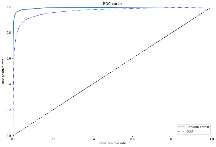
roc_auc_score(y_train_5,y_scores_forest)
0.9925669179297443
The Random Forest model is a clear improvement over the SGD in this case.
Training a multiclass classifier
One v All
Training works in much the same way, the SGD will create 10 models, similar to how we created our binary classifier to detect 5s, one for each number. This is the default for most algorithms.
sgd_clf.fit(X_train,y_train)
sgd_clf.predict([some_digit])
array([5.])
some_digit_scores = sgd_clf.decision_function([some_digit])
some_digit_scores
array([[ -41786.61539188, -132632.74409099,  -47807.94492258,
         -24820.12021653, -111452.34755583,    4702.12446528,
        -199410.47118134,  -45622.13582631,  -70711.0599054 ,
        -140366.69430641]])
This array of scores correspond to the 10 classes, the highest scores, 5 in this case, will be selected as the predicted answer.
sgd_clf.classes_
array([0., 1., 2., 3., 4., 5., 6., 7., 8., 9.])
One V One
Using one v one creates a binary classifier for each pair of digits, 0v1, 0v2, 1v2 etc creating 45 classifiers in all. Support Vector Machines(SVM) will use this by default as their training time increases exponentially with larger training sets, so many smaller sets is preferred. Any model can be forced to use OvO or OvA.
from sklearn.multiclass import OneVsOneClassifier

ovo_clf = OneVsOneClassifier(SGDClassifier(max_iter=1000,tol=1e-3,random_state=42))
ovo_clf.fit(X_train,y_train)
ovo_clf.predict([some_digit])
array([5.])
len(ovo_clf.estimators_)
45
Evaluating classifiers
Using cross_val_score
names = ['RandomForest','SGD OvA','SGD OvO']
classifiers = [forest,sgd_clf,ovo_clf]

for name, classifier in zip(names,classifiers):
    print('Cross val score for ',name,' : ',cross_val_score(classifier,X_train,y_train,scoring='accuracy'))
Cross val score for  RandomForest  :  [0.93936213 0.93964698 0.93879082]
Cross val score for  SGD OvA  :  [0.84918016 0.87434372 0.87788168]
Cross val score for  SGD OvO  :  [0.91821636 0.90894545 0.90983648]
Model tuning
Tuning the model and input features to try and improve performance
Scaling features
from sklearn.preprocessing import StandardScaler

scaler = StandardScaler()
X_train_scaled = scaler.fit_transform(X_train.astype(np.float64))

for name, classifier in zip(names,classifiers):
    print('Scaled cross val score for ',name,' : ',
          cross_val_score(classifier,X_train_scaled,y_train,scoring='accuracy'))
Scaled cross val score for  RandomForest  :  [0.93941212 0.93969698 0.9386908 ]
Scaled cross val score for  SGD OvA  :  [0.89997001 0.90144507 0.90683603]
Scaled cross val score for  SGD OvO  :  [0.91776645 0.9159958  0.9193379 ]
RandomizedSearchCV
Using our best model, we will run through 10 iterations to try and find optimal parameters. Here I have created a custom randomized search CV to view the scores as each iteration finishes, storing the results and parameters in a dataframe sorted by mean CV score.
import itertools
import pandas as pd

def random_search_cv(param_grid,X,y,n_iter=10):
    keys,values = zip(*param_grid.items())
    combinations = [dict(zip(keys, v)) for v in itertools.product(*values)]
    results = pd.DataFrame(columns=['mean_cv_score','params','iteration'],index=list(range(n_iter)))
    for i in range(n_iter):
        params = np.random.choice(combinations)
        f = RandomForestClassifier(**params)
        score = cross_val_score(f,X,y,cv=3)
        results.loc[i,'mean_cv_score']=score.mean()
        results.loc[i,'params']=str(params)
        results.loc[i,'iteration']=i
        print('Round : {}   Score : {}'.format(i,score))
        results.sort_values('mean_cv_score',inplace=True)
        results.reset_index()
    return results
param_grid = {'n_estimators' : np.arange(10,200,10),'bootstrap' : [True,False]}
results = random_search_cv(param_grid,X_train,y_train,n_iter=10)
Round : 0   Score : [0.96495701 0.96554828 0.96639496]
Round : 1   Score : [0.95940812 0.9579479  0.96044407]
Round : 2   Score : [0.96440712 0.96369818 0.96444467]
Round : 3   Score : [0.96540692 0.96534827 0.966695  ]
Round : 4   Score : [0.96925615 0.97074854 0.97074561]
Round : 5   Score : [0.96910618 0.96979849 0.96949542]
Round : 6   Score : [0.96340732 0.96304815 0.96359454]
Round : 7   Score : [0.96480704 0.96464823 0.96629494]
Round : 8   Score : [0.96540692 0.9659983  0.96704506]
Round : 9   Score : [0.96890622 0.96979849 0.97019553]
results.head()
| mean_cv_score | params | iteration | |
|---|---|---|---|
| 1 | 0.959267 | {'n_estimators': 30, 'bootstrap': True} | 1 |
| 6 | 0.96335 | {'n_estimators': 60, 'bootstrap': True} | 6 |
| 2 | 0.964183 | {'n_estimators': 70, 'bootstrap': True} | 2 |
| 7 | 0.96525 | {'n_estimators': 30, 'bootstrap': False} | 7 |
| 0 | 0.965633 | {'n_estimators': 100, 'bootstrap': True} | 0 |
Error evaluation
Confusion Matrix
Looking at the confusion matrix we can observe what types of errors our model is making in order to find ways to improve it.
y_train_pred = cross_val_predict(forest, X_train_scaled, y_train, cv=3)
conf_mx = confusion_matrix(y_train,y_train_pred)
conf_mx
array([[5809,    1,   11,    7,    8,   15,   33,    4,   28,    7],
       [   1, 6620,   37,   17,   18,   12,    9,   11,   12,    5],
       [  50,   23, 5617,   42,   41,   10,   34,   55,   71,   15],
       [  21,   30,  146, 5623,    9,  117,    3,   52,   91,   39],
       [  21,   13,   46,    9, 5518,    8,   36,   18,   27,  146],
       [  60,   11,   26,  186,   27, 4948,   62,    5,   58,   38],
       [  55,   14,   25,    3,   29,   72, 5701,    0,   19,    0],
       [  14,   36,   87,   22,   69,    4,    0, 5939,   10,   84],
       [  39,   60,  117,  121,   49,  103,   52,   24, 5215,   71],
       [  33,   20,   37,   97,  196,   50,    4,   93,   53, 5366]])
Image representation of confusion matrix
plt.figure(figsize=(12,8))
plt.matshow(conf_mx,cmap=plt.cm.gray,fignum=1)
<matplotlib.image.AxesImage at 0x7f58a86413c8>
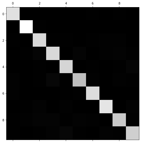
Still very hard to understand what is going on, we are currently looking at the number of absolute errors which will be unrepresentative if some features have few instances. Normalizing by dividing by each value by the number of images in the class will leave us with the error rate instead.
Normed confusion matrix
By also filling the diagonals we are left with only the errors.
row_sums = conf_mx.sum(axis=1, keepdims=True)
norm_conf_mx= conf_mx /row_sums

np.fill_diagonal(norm_conf_mx, 0)
plt.figure(figsize=(8,8))
plt.matshow(norm_conf_mx, cmap=plt.cm.gray,fignum=1)
plt.show()
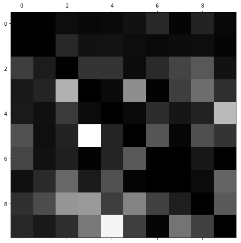
The light areas show where the errors are most profound, columns 8 and 9 are bright, meaning digits often get confused for being 8 or 9. The rows are also quite bright for 8 amd 9, meaning 8s and 9s are often confused for other digits.
3s and 5s are also confused for each other a lot.
To address these problems we could add another feature - number of closed loops - and write an algorithm to detect these. We could also use image preprocessing software to make these and other features stand out more clearly to help our new or existing model detect the differences.
Testing our model on the test set
If we were going to add features, get more training data or further fine tune our model we would do this now. But for the purposes of this project, having tested several classifiers, ran tests scaling the input features and tuned the model parameters I am ready to use the best performing model to predict on the test set.
import ast
from sklearn.metrics import accuracy_score

best_params = ast.literal_eval(results['params'][0])
model = RandomForestClassifier(**best_params)
model.fit(X_train,y_train)

predictions = model.predict(X_test)

print('Accuracy score for our final model : ',accuracy_score(y_test,predictions))
Accuracy score for our final model : 0.9704
97% accuracy is a big improvement over our initial model
Conclusion and next steps
We have greatly improved our accuracy by several percentage points over our inital multiclass model, however ther are still many steps that could have be taken to improve it before we used the test set.
Grid search CV
Having searched the hyperparameter space using a random search we can now hone in on the best models with a more focused search around those values attempting to improve our scores.
Data augmentation
Not having any more training data available, we could create “new” images using our training set, rotating or shifting the images in different directions by just 1 pixel will create many different images for our models to train on.
Error evaluation
Repeating the error analysis, we could create an algorithm that detects closed loops or other distinct patterns, creating new features that many help our model reduce errors in problem areas.
It should be noted however that any further changes to our model now the test set has been used will lead to overfitting the test set and not generalizing well to new data.