Wine Quality
A study into wine quality, the task is to assess which is the most important feature of wine when a quality rating is being assigned by a taster. Features are a variety of physiochemical readings and the target variable ‘quality’ is a sensory reading with a scale of 0-10.
The dataset was acquired courtesy of:
P. Cortez, A. Cerdeira, F. Almeida, T. Matos and J. Reis. Modeling wine preferences by data mining from physicochemical properties. In Decision Support Systems, Elsevier, 47(4):547-553, 2009.
And is available for download at the UCI machine learning repository here.
White wine
import pandas as pd

white = pd.read_csv('winequality-white.csv',sep=';')
white.head()
| fixed acidity | volatile acidity | citric acid | residual sugar | chlorides | free sulfur dioxide | total sulfur dioxide | density | pH | sulphates | alcohol | quality | |
|---|---|---|---|---|---|---|---|---|---|---|---|---|
| 0 | 7.0 | 0.27 | 0.36 | 20.7 | 0.045 | 45.0 | 170.0 | 1.0010 | 3.00 | 0.45 | 8.8 | 6 |
| 1 | 6.3 | 0.30 | 0.34 | 1.6 | 0.049 | 14.0 | 132.0 | 0.9940 | 3.30 | 0.49 | 9.5 | 6 |
| 2 | 8.1 | 0.28 | 0.40 | 6.9 | 0.050 | 30.0 | 97.0 | 0.9951 | 3.26 | 0.44 | 10.1 | 6 |
| 3 | 7.2 | 0.23 | 0.32 | 8.5 | 0.058 | 47.0 | 186.0 | 0.9956 | 3.19 | 0.40 | 9.9 | 6 |
| 4 | 7.2 | 0.23 | 0.32 | 8.5 | 0.058 | 47.0 | 186.0 | 0.9956 | 3.19 | 0.40 | 9.9 | 6 |
white.info()
<class 'pandas.core.frame.DataFrame'>
RangeIndex: 4898 entries, 0 to 4897
Data columns (total 12 columns):
fixed acidity           4898 non-null float64
volatile acidity        4898 non-null float64
citric acid             4898 non-null float64
residual sugar          4898 non-null float64
chlorides               4898 non-null float64
free sulfur dioxide     4898 non-null float64
total sulfur dioxide    4898 non-null float64
density                 4898 non-null float64
pH                      4898 non-null float64
sulphates               4898 non-null float64
alcohol                 4898 non-null float64
quality                 4898 non-null int64
dtypes: float64(11), int64(1)
memory usage: 459.3 KB
White wine features are all floats, the target is an integer and there are no missing values to deal with.
%matplotlib inline
import matplotlib.pyplot as plt

plt.figure(figsize=(32,22))
for i in range(1, white.shape[1]+1):
    plt.subplot(4,3,i)
    plt.title(white.columns[i-1],size=12)
    plt.hist(white.iloc[:,i-1], bins=30)

plt.show()
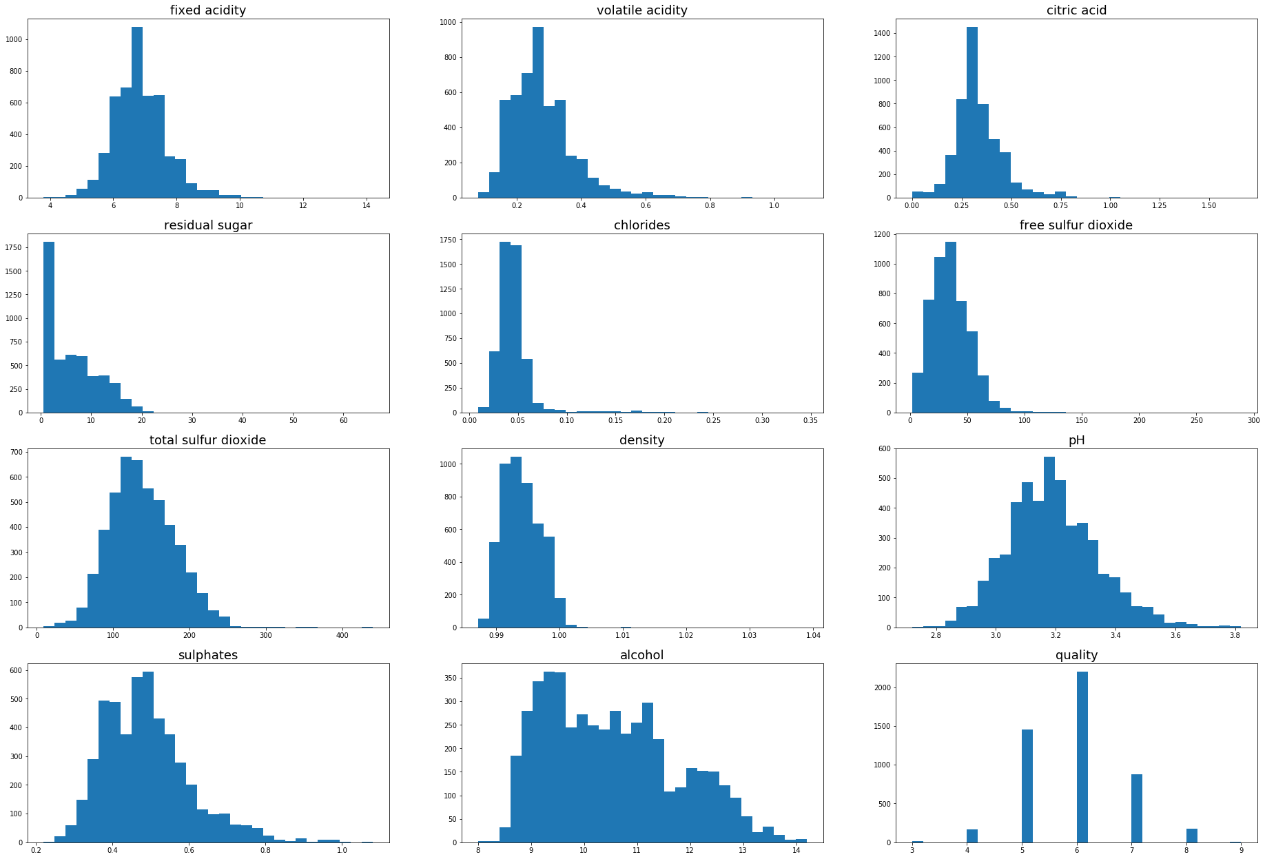
The physio chemical features contain a variety of distributions, there appear to be several outlier values for the majority of the features that could be detected and removed to aid in training a predictive model. There is an excellent explanation on why RandomForests are not immune to being swayed by outliers in the answer to this stackoverflow post.
As the target variable is integers between 0 and 10 we can approach this as either a classification or regression problem. The classes are however related, an incorrect prediction of a 6 for a wine rated 7 is a very different result to a prediction of 1 for the same wine so we will use a regression model.
corr = white.corr()
corr['quality'].abs().sort_values(ascending=False)
quality                 1.000000
alcohol                 0.435575
density                 0.307123
chlorides               0.209934
volatile acidity        0.194723
total sulfur dioxide    0.174737
fixed acidity           0.113663
pH                      0.099427
residual sugar          0.097577
sulphates               0.053678
citric acid             0.009209
free sulfur dioxide     0.008158
Name: quality, dtype: float64
Correlation does not guarantee causation, but the two features most correlated with the target are alcohol and density.
Using SKlearns RandomForestRegressor we can assess feature importance, during training of the model each feature will be ranked on the total decrease in node impurity (weighted by the probability of reaching that node which is approximated by the proportion of samples reaching that node) averaged over all trees of the ensemble.
import numpy as np
from sklearn.ensemble import RandomForestRegressor


def feature_importance(X,y):
    feature_importances = np.zeros(X.shape[1])

    for i in range(2):
        model = RandomForestRegressor(n_estimators=100,random_state=i)
        model.fit(X,y)
        feature_importances += model.feature_importances_

    feature_importances = feature_importances / 2

    return sorted(zip(feature_importances, X.columns),reverse=True)
X = white.drop(columns=['quality'])
y = white.quality

white_mdi = feature_importance(X,y)
white_mdi
[(0.24274913624324615, 'alcohol'),
 (0.12376860851037971, 'volatile acidity'),
 (0.11598499580507493, 'free sulfur dioxide'),
 (0.07040292142420893, 'pH'),
 (0.06976662436877715, 'total sulfur dioxide'),
 (0.06966357780105313, 'residual sugar'),
 (0.06277948391507257, 'chlorides'),
 (0.06233679219452094, 'sulphates'),
 (0.061924065377629206, 'density'),
 (0.06066232339017698, 'fixed acidity'),
 (0.059961470969860264, 'citric acid')]
Alcohol is ranked almost twice as important as any other feature of white wine.
Assessing importance via mean decrease accuracy we can compare results with the previous test. Mean decrease accuracy works via shuffling all of the values of a feature, effectively destroying its predictive power but not affecting the distritbution of the dataset. Accuracy scores are then compared between the shuffled and unshuffled data, the features with the highest scores are theoretically the most important as the accuracy decrease is greatest when shuffling that feature.
from sklearn.model_selection import ShuffleSplit
from sklearn.metrics import r2_score

def mean_decrease_accuracy(X,y):
    shuffler = ShuffleSplit(n_splits=3, test_size=0.3)
    total_scores = np.zeros(X.shape[1])

    for train_idx, test_idx in shuffler.split(X):
        scores = []
        model = RandomForestRegressor(n_estimators=100)
        model.fit(X.loc[train_idx,:],y[train_idx])
        predictions = model.predict(X.loc[test_idx,:])
        r2 = r2_score(y[test_idx],predictions)
        for i in range(X.shape[1]):
            X_shuffle = X.copy()
            np.random.shuffle(X[X.columns[i]])
            model = RandomForestRegressor(n_estimators=100)
            model.fit(X_shuffle.loc[train_idx,:],y[train_idx])
            pred = model.predict(X_shuffle.loc[test_idx,:])
            r2_shuffle = r2_score(y[test_idx], pred)
            score = ((r2 - r2_shuffle) / r2)
            scores.append(score)
        total_scores += scores

    mean_scores = total_scores / 3

    return sorted(zip(mean_scores, X.columns),reverse=True)
white_mda = mean_decrease_accuracy(X,y)
white_mda
[(0.3981994161296054, 'total sulfur dioxide'),
 (0.3310424321954958, 'pH'),
 (0.3188281671857857, 'sulphates'),
 (0.2932985343693217, 'density'),
 (0.09132366976518407, 'alcohol'),
 (0.06272617799945564, 'citric acid'),
 (0.044638614719226526, 'chlorides'),
 (0.02573899375065399, 'free sulfur dioxide'),
 (0.020442684261677824, 'residual sugar'),
 (-0.05197866211717678, 'fixed acidity'),
 (-0.10092189745284881, 'volatile acidity')]
Four features, ‘total sulfur dioxide’, ‘pH’, ‘sulphates’ and ‘density’ rank much higher than the other features. Permuting the values of ‘Fixed acidity’ and ‘volalite acidity’ actually improved the models predictive power, suggesting they only add noise to the model.
Red wine
red = pd.read_csv('winequality-red.csv',sep=';')
plt.figure(figsize=(32,22))
for i in range(1, red.shape[1]+1):
    plt.subplot(4,3,i)
    plt.title(red.columns[i-1],size=12)
    plt.hist(red.iloc[:,i-1], bins=20)

plt.show()
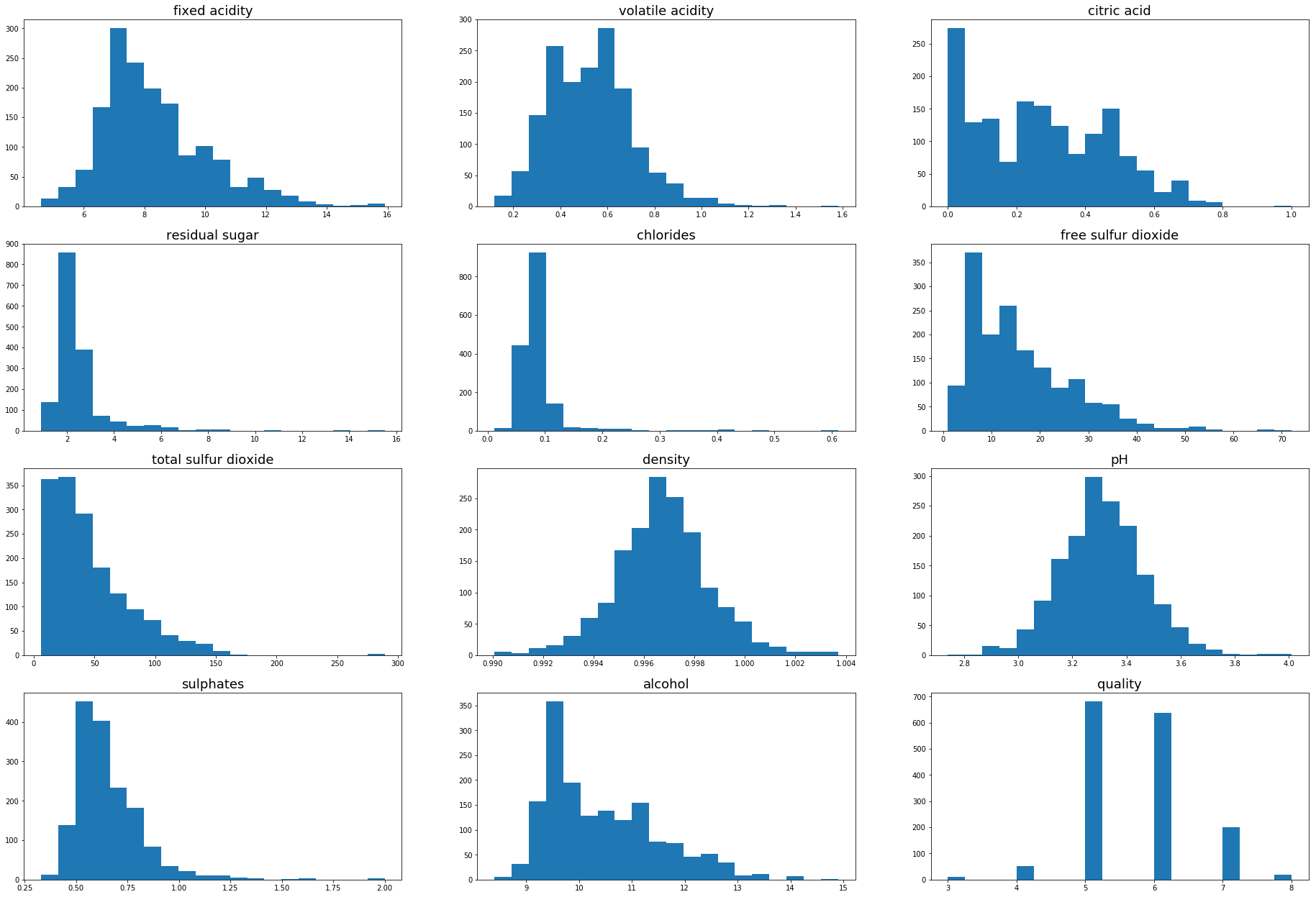
Much of the distributions of red wine are similar to that of white, the dataset does however seem to be less affected by outliers than the white wine.
red_corr = red.corr()
red_corr['quality'].abs().sort_values(ascending=False)
quality                 1.000000
alcohol                 0.476166
volatile acidity        0.390558
sulphates               0.251397
citric acid             0.226373
total sulfur dioxide    0.185100
density                 0.174919
chlorides               0.128907
fixed acidity           0.124052
pH                      0.057731
free sulfur dioxide     0.050656
residual sugar          0.013732
Name: quality, dtype: float64
Alcohol is again the most correlated feature.
X = red.drop(columns=['quality'])
y = red['quality']
red_mdi = feature_importance(X,y)
red_mdi
[(0.2717331877872253, 'alcohol'),
 (0.13786812417845237, 'sulphates'),
 (0.13245695103428867, 'volatile acidity'),
 (0.07939452142752387, 'total sulfur dioxide'),
 (0.06296083156468851, 'chlorides'),
 (0.0593168265853386, 'pH'),
 (0.05489868089262883, 'residual sugar'),
 (0.05295107593878534, 'density'),
 (0.052208732935507464, 'fixed acidity'),
 (0.04852153541977636, 'free sulfur dioxide'),
 (0.04768953223578466, 'citric acid')]
Ranked on mean decrease impurity alcohol is also the most important feature of red wine.
red_mda = mean_decrease_accuracy(X,y)
red_mda
[(0.15922150556809037, 'alcohol'),
 (0.11170131395272541, 'residual sugar'),
 (0.04892525208494835, 'volatile acidity'),
 (-0.01350363867285372, 'sulphates'),
 (-0.033861684440428474, 'free sulfur dioxide'),
 (-0.040502222962895594, 'pH'),
 (-0.060019863084332103, 'citric acid'),
 (-0.06262756184365433, 'fixed acidity'),
 (-0.14358225948266734, 'density'),
 (-0.17919731153872898, 'chlorides'),
 (-0.2063921978450319, 'total sulfur dioxide')]
Alcohol also ranks as the most important feature when assessing importances using the ‘OOB’ mean decrease accuracy method.
Conclusion
It is unclear after the two tests performed in this report which is the most important factor in determining white wine quality, alcohol content performs highly on the first modelling of feature importance. It is however beaten by four other features on the mean decrease accuracy test, more training data or different evaluation metrics may give a clearer picture.
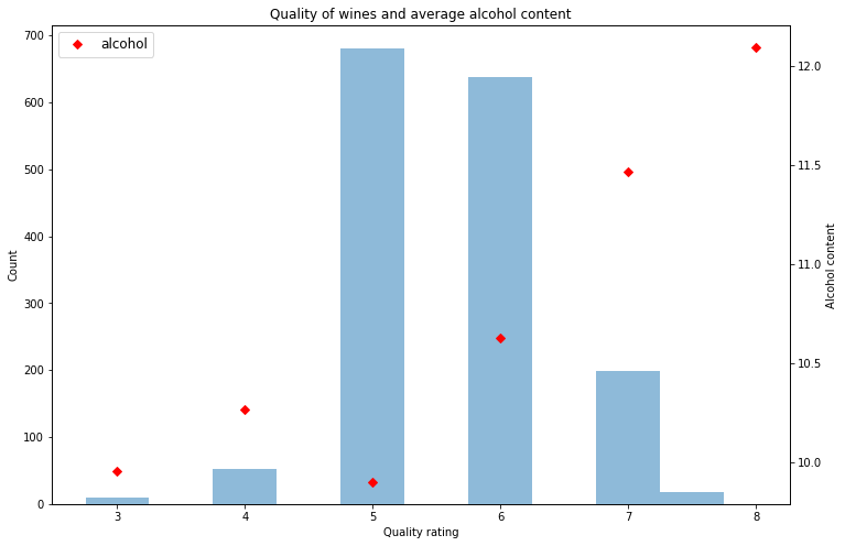
For red wine there is no question that using the dataset, metrics and methodology above that alcohol is the most important feature in determining the quality rating of the wine. What is not covered in this study is whether wine that is more expenisve and expected to be of a better quality also contains a higher percentage of alcohol.
As shown in the chart below the general trend of more alcohol equals higher rating is clear in the red wine dataset.
fig, ax1 = plt.subplots(figsize=(12,8))
ax1.hist(red.quality,align='left',alpha=0.5)
ax1.set_title('Quality of wines and average alcohol content')
ax1.set_xlabel('Quality rating')
ax1.set_ylabel('Count')
ax2 = ax1.twinx()
ax2.set_ylabel('Alcohol content')
ax2.plot(red.groupby('quality')['alcohol'].mean(),'D',color='red')
plt.legend(fontsize=12)
<matplotlib.legend.Legend at 0x7fe7b40cc2e8>